
Anomaly Detection for Predictive maintenance- Building autoregressive model
An auto-regressive model predicts time series values by a linear combination of its past values. It assumes that the time series shows aut-correlation and that the past value is correlated with the current value. The model will be able to predict the next sample in the time series when the system works properly. The error between the real sample and the predicted sample can then tell us something about the underlying system’s condition.Vector Auto-Regressive (VAR) Models for Multivariate Time Series Forecasting

Contents:
Train the Model
Steps to train
Test the Model
Deployment
Conclusion We train an auto-regressive model using the linear regression algorithm.
yt = c+φ1yt-1 + φ2yt-2+…+φpyt-p + εt,
Where yt is the target columnyt
-1, yt-2, …,yt-p are the predictor columns i.e. past values of yt up to the lag p
φ1, φ2, …,φ3 are the regression coefficients, and
εt is the white noise error term
Training the model:
We use the same data that was used for EDA for model training. The information is divided into three time windows (training, upkeep, and test), each of which is determined by the rotor breakdown date, which is July 21, 2008:
Training window from January to August 2007
Maintenance window from September 2007 to July 21, 2008
Test window after July 22, 2008
Steps to train:
1.We train the models on the data from the training window. We loop over all 313 columns in the data representing the amplitude values on the single frequency bands.
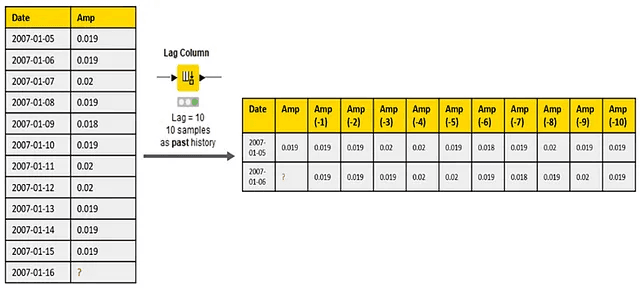
2.For each column at a time, we generate the predictor columns with the Lag Column node that puts the data in the p previous rows into p new columns.
3.The transformed table contains the target column and a column for each past value at a different lag 1,2,…,p.
4.These are the predictor columns of the auto-regressive model called xx (-1), xx (-2), …, xx (-p), where xx refers to the name of the target column and the number in the brackets refers to the lag as shown in the figure.
5.Next, we train a linear regression model on the transformed data and save the model as a PMML file.
6.This model will be used later to predict future values.
7.We also perform in-sample prediction, that is we apply the model to the training data, and save the prediction error statistics.
Lag columnFull knime workflow to build the auto-regressive modelinside error-stat meta node
the output of error stat
Testing the model:
We want to know the out-sample prediction performance of our model, so we predict the data from the maintenance window.
We loop over all 313 columns in the maintenance window and predict the values in it. We compare the predictions to the actual values and compare the prediction errors to the in-sample prediction errors.
Finally, we calculate 1st and 2nd-level alarms and visualize them.
Workflow for testing
Calculate 1st level alarm:
The 1st level errors are calculated by comparing the in-sample prediction errors (on the training set) and out-sample prediction errors (on the maintenance set).
We limit the boundaries for the normal behavior as average (avg) +/- 2*standard deviation (stddev) of the in-sample prediction.
1st level alarm
Calculating 2nd level alarm:
2nd level alarms are calculated as the average of the backward window of 21 1st-level alarms, which we can do with the Moving Aggregation node.
The backward window-based moving average substitutes the last sample of the window with the average value of the previous models in the same window.
The backward window approach is necessary to simulate real-life monitoring conditions, where past and current measures are available, but future measures are not.
The moving average operation smooths out all random peaks in the 1st level alarm time series, and produces peaks in the 2nd level alarm time series, only if the 1st level alarm peaks persist over time.
2nd level alarms
2nd level alarms
Line plot
We observe the evolution of the 2nd level alarm time series before the rotor breakdown in a line plot and a stacked area chart.
Figure 5 shows a line plot with the 2nd level alarms on multiple frequency bands of one sensor (SV3) through the maintenance window from September 2007 to July 21, 2008.
As we can see, in the first months of the maintenance window, hardly any alarms were raised.
However, starting in May 2008, about 3 months before the rotor breakdown on July 21, 2008, the second-level alarms were raised on all frequency bands. Especially the [200–300Hz] frequency band (the purple line) reacts strongly to the deteriorating rotor.
Stacked Area chart
Stacked area chart
The above Figure shows a stacked area chart with the cumulative 2nd level alarm across all frequency bands and all sensors through the maintenance window.
Here the earliest signs of the rotor malfunctioning can be tracked back as early as the beginning of March 2008. However, the change in the system became evident at the beginning of May 2008, especially in some frequency bands of some sensors (see [200–300] A7-SA1 time series with a green area).
Considering the rotor breakdown on July 21, 2008, this would have been a fairly advanced warning time! If we wanted to have an earlier/later sign of the rotor malfunctioning, we could change the thresholds for the 1st and 2nd level alarms, and make them less/more tolerant towards prediction errors.
Deployment• We know now that our alarm system starts bugging us before the rotor breakdown. What should we do?
We decide to notify mechanical support via email.
If it was more urgent, we could switch off the system immediately via a REST service.
Workflow for Deployment
The workflow is the same as the Anomaly Detection. Time Series AR Testing workflow.
Deployment workflow
Trigger Check-up if level 2 Alarm =1
If, level 2 alarm=1 then a workflow will be called to send an email to the concerned person to start a trigger checkup.
Trigger Check up
Call workflow node configuration
By using the call workflow node, the send_email_to_start_checkup workflow is called is executed.
Send_email_to_start_checkup workflow
Send email node configuration
The workflow we call is shown in the above figure. The Send Email node — as the name says — sends an email using a specified account on an SMTP host and its credentials. The other node in the workflow is a Container Input (variable) node. While this node is functionally not important, it is required to pass the data from the calling to the called workflow. Indeed, the Call Workflow (Table Based) node passes all the flow variables available at its input port to the Container Input (Variable) node. In summary, the Container Input (Variable) node is a bridge to transport the flow variables available at the caller node into the called workflow.
If we decided to, for example, switch off the system instead, we would only need to change the configuration of the Call Workflow (Table-based) node to trigger the execution of such a workflow. Otherwise, the deployment workflow would remain the same. Also notice that we triggered the execution of a local workflow from another local workflow. However, if we wrapped the workflow with the Container Input and Container Output nodes and deployed it to a KNIME Server, the workflow could be called from any external service
Conclusion
In this article, We built an auto-regressive model to predict the rotor breakdown. We categorized single remarkable prediction errors as 1st-level alarms and persisting 1st-level alarms as 2nd-level alarms.
We then tested the model on the maintenance window that ends in the rotor breakdown. In the deployment phase, we automatically emailed mechanical support if the 2nd level alarm was active.I hope this article was informative and provided you with the details you required. If you have any questions related to Knime Analytics, Machine Learning, and Deep Learning Documentation while reading the blog, message me on Instagram or Linkedin. Special credits to my team interns: Shreyas, Siddhid, Urvi, Kishan, Pratik.Thank you…
An auto-regressive model predicts time series values by a linear combination of its past values. It assumes that the time series shows aut-correlation and that the past value is correlated with the current value. The model will be able to predict the next sample in the time series when the system works properly. The error between the real sample and the predicted sample can then tell us something about the underlying system’s condition.Vector Auto-Regressive (VAR) Models for Multivariate Time Series Forecasting
Contents:
Train the Model
Steps to train
Test the Model
Deployment
Conclusion We train an auto-regressive model using the linear regression algorithm.
yt = c+φ1yt-1 + φ2yt-2+…+φpyt-p + εt,
Where yt is the target columnyt
-1, yt-2, …,yt-p are the predictor columns i.e. past values of yt up to the lag p
φ1, φ2, …,φ3 are the regression coefficients, and
εt is the white noise error term
Training the model:
We use the same data that was used for EDA for model training. The information is divided into three time windows (training, upkeep, and test), each of which is determined by the rotor breakdown date, which is July 21, 2008:
Training window from January to August 2007
Maintenance window from September 2007 to July 21, 2008
Test window after July 22, 2008
Steps to train:
1.We train the models on the data from the training window. We loop over all 313 columns in the data representing the amplitude values on the single frequency bands.
2.For each column at a time, we generate the predictor columns with the Lag Column node that puts the data in the p previous rows into p new columns.
3.The transformed table contains the target column and a column for each past value at a different lag 1,2,…,p.
4.These are the predictor columns of the auto-regressive model called xx (-1), xx (-2), …, xx (-p), where xx refers to the name of the target column and the number in the brackets refers to the lag as shown in the figure.
5.Next, we train a linear regression model on the transformed data and save the model as a PMML file.
6.This model will be used later to predict future values.
7.We also perform in-sample prediction, that is we apply the model to the training data, and save the prediction error statistics.
Lag columnFull knime workflow to build the auto-regressive modelinside error-stat meta node
the output of error stat
Testing the model:
We want to know the out-sample prediction performance of our model, so we predict the data from the maintenance window.
We loop over all 313 columns in the maintenance window and predict the values in it. We compare the predictions to the actual values and compare the prediction errors to the in-sample prediction errors.
Finally, we calculate 1st and 2nd-level alarms and visualize them.
Workflow for testing
Calculate 1st level alarm:
The 1st level errors are calculated by comparing the in-sample prediction errors (on the training set) and out-sample prediction errors (on the maintenance set).
We limit the boundaries for the normal behavior as average (avg) +/- 2*standard deviation (stddev) of the in-sample prediction.
1st level alarm
Calculating 2nd level alarm:
2nd level alarms are calculated as the average of the backward window of 21 1st-level alarms, which we can do with the Moving Aggregation node.
The backward window-based moving average substitutes the last sample of the window with the average value of the previous models in the same window.
The backward window approach is necessary to simulate real-life monitoring conditions, where past and current measures are available, but future measures are not.
The moving average operation smooths out all random peaks in the 1st level alarm time series, and produces peaks in the 2nd level alarm time series, only if the 1st level alarm peaks persist over time.
2nd level alarms
2nd level alarms
Line plot
We observe the evolution of the 2nd level alarm time series before the rotor breakdown in a line plot and a stacked area chart.
Figure 5 shows a line plot with the 2nd level alarms on multiple frequency bands of one sensor (SV3) through the maintenance window from September 2007 to July 21, 2008.
As we can see, in the first months of the maintenance window, hardly any alarms were raised.
However, starting in May 2008, about 3 months before the rotor breakdown on July 21, 2008, the second-level alarms were raised on all frequency bands. Especially the [200–300Hz] frequency band (the purple line) reacts strongly to the deteriorating rotor.
Stacked Area chart
Stacked area chart
The above Figure shows a stacked area chart with the cumulative 2nd level alarm across all frequency bands and all sensors through the maintenance window.
Here the earliest signs of the rotor malfunctioning can be tracked back as early as the beginning of March 2008. However, the change in the system became evident at the beginning of May 2008, especially in some frequency bands of some sensors (see [200–300] A7-SA1 time series with a green area).
Considering the rotor breakdown on July 21, 2008, this would have been a fairly advanced warning time! If we wanted to have an earlier/later sign of the rotor malfunctioning, we could change the thresholds for the 1st and 2nd level alarms, and make them less/more tolerant towards prediction errors.
Deployment• We know now that our alarm system starts bugging us before the rotor breakdown. What should we do?
We decide to notify mechanical support via email.
If it was more urgent, we could switch off the system immediately via a REST service.
Workflow for Deployment
The workflow is the same as the Anomaly Detection. Time Series AR Testing workflow.
Deployment workflow
Trigger Check-up if level 2 Alarm =1
If, level 2 alarm=1 then a workflow will be called to send an email to the concerned person to start a trigger checkup.
Trigger Check up
Call workflow node configuration
By using the call workflow node, the send_email_to_start_checkup workflow is called is executed.
Send_email_to_start_checkup workflow
Send email node configuration
The workflow we call is shown in the above figure. The Send Email node — as the name says — sends an email using a specified account on an SMTP host and its credentials. The other node in the workflow is a Container Input (variable) node. While this node is functionally not important, it is required to pass the data from the calling to the called workflow. Indeed, the Call Workflow (Table Based) node passes all the flow variables available at its input port to the Container Input (Variable) node. In summary, the Container Input (Variable) node is a bridge to transport the flow variables available at the caller node into the called workflow.
If we decided to, for example, switch off the system instead, we would only need to change the configuration of the Call Workflow (Table-based) node to trigger the execution of such a workflow. Otherwise, the deployment workflow would remain the same. Also notice that we triggered the execution of a local workflow from another local workflow. However, if we wrapped the workflow with the Container Input and Container Output nodes and deployed it to a KNIME Server, the workflow could be called from any external service
Conclusion
In this article, We built an auto-regressive model to predict the rotor breakdown. We categorized single remarkable prediction errors as 1st-level alarms and persisting 1st-level alarms as 2nd-level alarms.
We then tested the model on the maintenance window that ends in the rotor breakdown. In the deployment phase, we automatically emailed mechanical support if the 2nd level alarm was active.I hope this article was informative and provided you with the details you required. If you have any questions related to Knime Analytics, Machine Learning, and Deep Learning Documentation while reading the blog, message me on Instagram or Linkedin. Special credits to my team interns: Shreyas, Siddhid, Urvi, Kishan, Pratik.Thank you…