Implementing Random Erasing upon PostDam Dataset
Random Erasing is a new data augmentation method for training the convolutional neural network (CNN).
Random Erasing
Contents:
Introduction to Random Erasing
Steps to achieve Random Erasing
Intraining, Random Erasing randomly selects a rectangle region in an image and erases its pixels with random values. In this process, training images with various levels of occlusion are generated, which reduces the risk of over-fitting and makes the model robust to occlusion. Random Erasing is parameter learning free, easy to implement, and can be integrated with most of the CNN-based recognition models.
Albeit simple, Random Erasing is complementary to commonly used data augmentation techniques such as random cropping and flipping, and yields consistent improvement over strong baselines in image classification, object detection, and person re-identification.
So, will perform step by step process and achieve Random Erasing from a well-known Potsdam dataset.
Dataset link:
Let’s hop in,
Step 1: To use Google Colab, the company’s most popular data science tool, we must first join in using our Google accounts. To make advantage of the GPU capabilities, we are utilizing Google Colab.
Step 2: Once we have the Colab in our possession, we mount the drive so that we may use the data that is on it. The corresponding photo is shown below.
Colab
Step 3: We will now download the dataset directly to the disc. The corresponding photo is shown below. The snippet below shows how to get data from a source and unzip it into a certain directory.
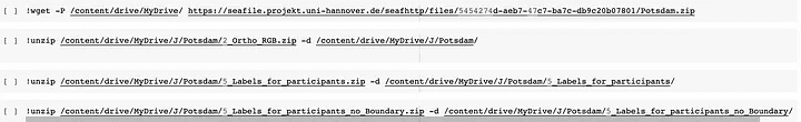
Dataset
Step 4: After receiving the dataset, I’ll download the relevant packages, import them into the colab, and then proceed with the processing. The corresponding photo is shown below.
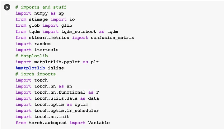
Packages
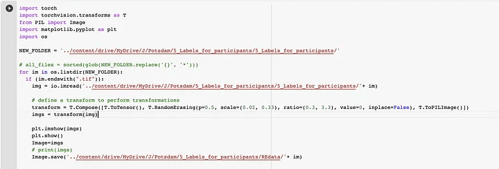
Step 5: For our Potsdam dataset, we will use the random erasing function from Pytorch itself. So, in essence, we’ll create another Random Erasing dataset and utilize it for additional training. As a result, we are creating and saving the dataset in a particular place.
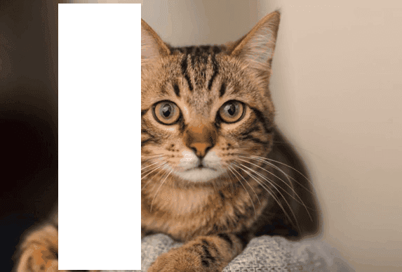
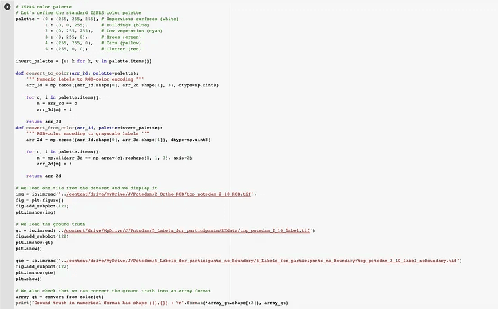
Step 6: Here, we will visualize the just-created random erasing dataset. The relevant photo is shown below. Let’s first examine if we can get the dataset and figure out what’s going on. Scikit-Image is what we’re using to manipulate images. We must create a color palette that can transfer the label id to its RGB color since the ISPRS dataset is stored with ground truth in the RGB format. To convert from numbers to colors and vice versa, we construct two helper functions.
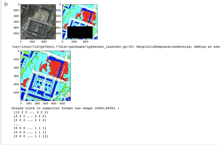
The above code snippet gives output like the below image.
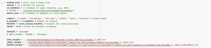
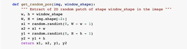
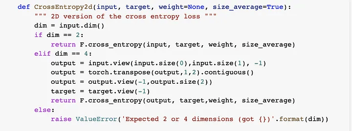
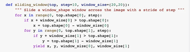
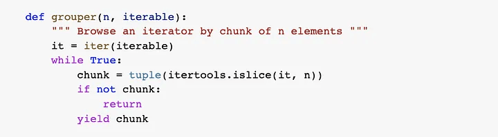
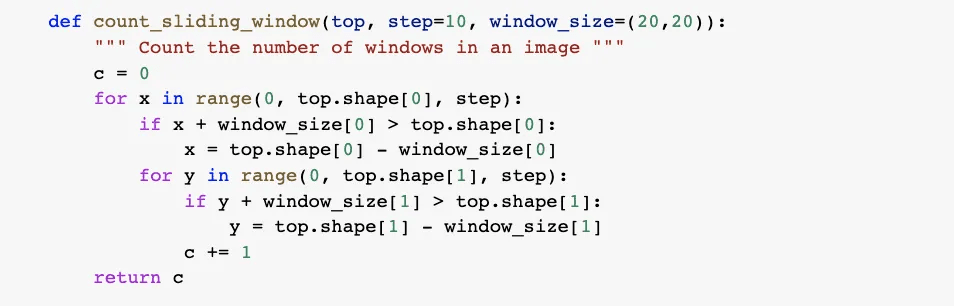
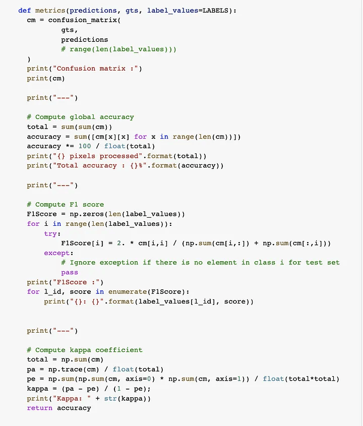
Step 7: Here, At this point, we need to define a bunch of utils function for the smooth processing
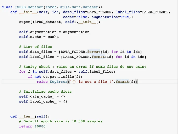
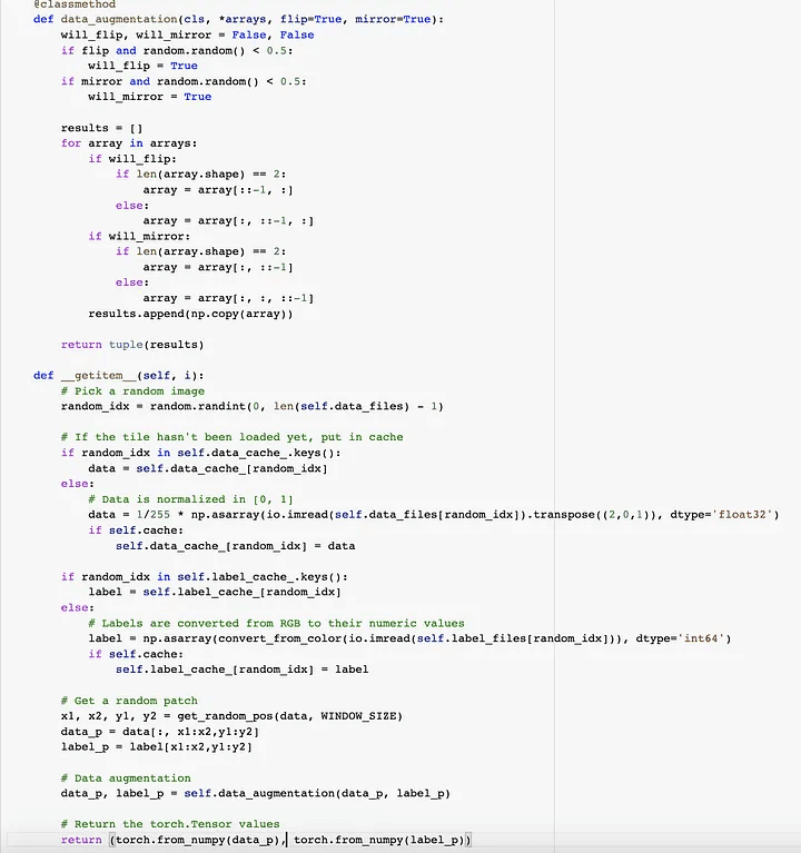
Step 8: Now we are loading the dataset, We define a PyTorch dataset (torch.utils.data.Dataset) that loads all the tiles in memory and performs random sampling. Tiles are stored in memory on the fly. The dataset also performs random data augmentation (horizontal and vertical flips) and normalizes the data in [0, 1].
So, we have defined a class and within it, data augmentation functions like flip, rotate, etc. Below is the snippet for the same.
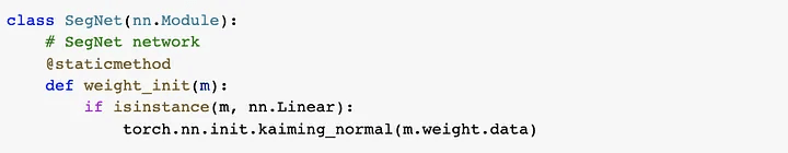
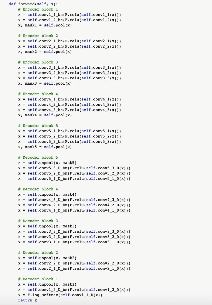
Step 9: Now, the time comes for network definition for CNN, We can now define the Fully Convolutional network based on the SegNet architecture. We could use any other network as a drop-in replacement, provided that the output has dimensions (N_CLASSES, W, H) where W and H are the sliding window dimensions (i.e. the network should preserve the spatial dimensions).
Step 10: We can now instantiate the network using the specified parameters. By default, the weights will be initialized using the policy.
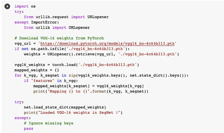
Step 11: We download and load the pre-trained weights from VGG-16 on ImageNet. This step is optional but it makes the network converge faster. We skip the weights from VGG-16 that have no counterpart in SegNet.
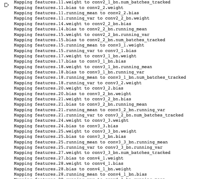
Below is the output of the above snippet.
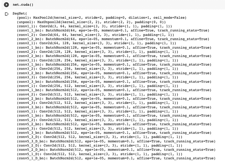
Step 12: Now, we load the network on GPU. Follow the below link till Step 5, Link for GPU in the Colab:
https://www.geeksforgeeks.org/how-to-run-cuda-c-c-on-jupyter-notebook-in-google-colaboratory/
How To Run CUDA C/C++ on Jupyter notebook in Google Colaboratory - GeeksforGeeks
What is CUDA? CUDA is a model created by Nvidia for a parallel computing platform and application programming interface…
www.geeksforgeeks.org
And then write below code snippet.
Step 13: Now below is the code snippet with output for Cuda for training the CNN.
Step 14: Check the image below to see if the GPU is active.
Step 15: Now we establish a train/test divide. You must modify the code to gather all filenames if you wish to utilize another dataset. In our scenario, the demo has a fixed train/test split.
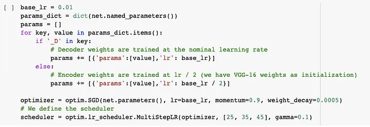
Step 16: We are now designing the optimizer. We use the standard Stochastic Gradient Descent algorithm to optimize the network’s weights. The encoder is trained at half the learning rate of the decoder, as we rely on the pre-trained VGG-16 weights.
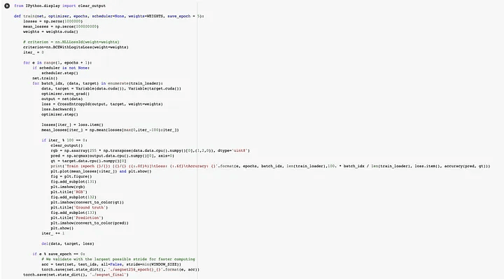
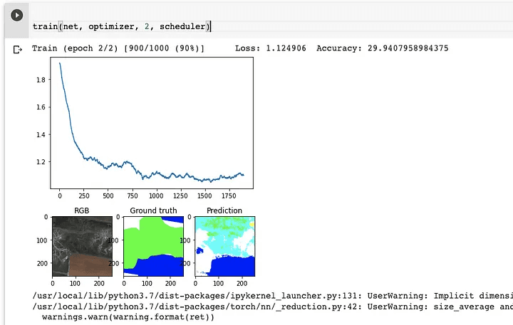
Step 17: Let’s progressively raise once the network has trained for two epochs. The loss plot and an example inference are updated on the matplotlib graph on a regular basis.
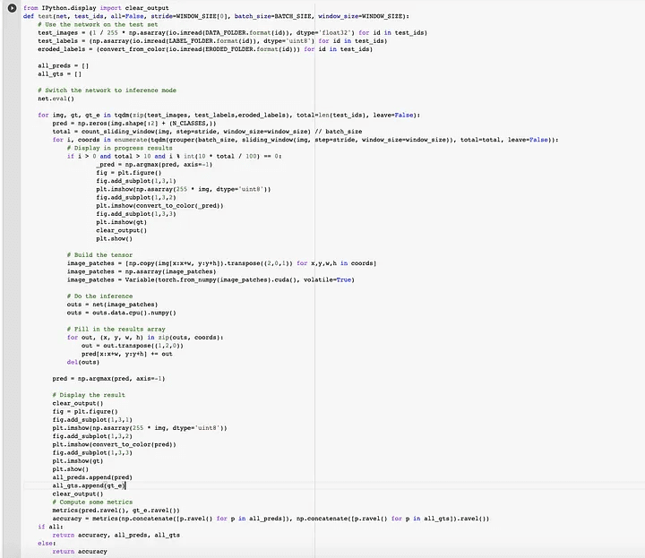
Step 18: Now that the training has ended, we can load the final weights and test the network using a reasonable stride, e.g. half or a quarter of the window size. Inference time depends on the chosen stride, e.g. a step size of 32 (75% overlap) will take ~30 minutes, but no overlap will take only one minute or two.
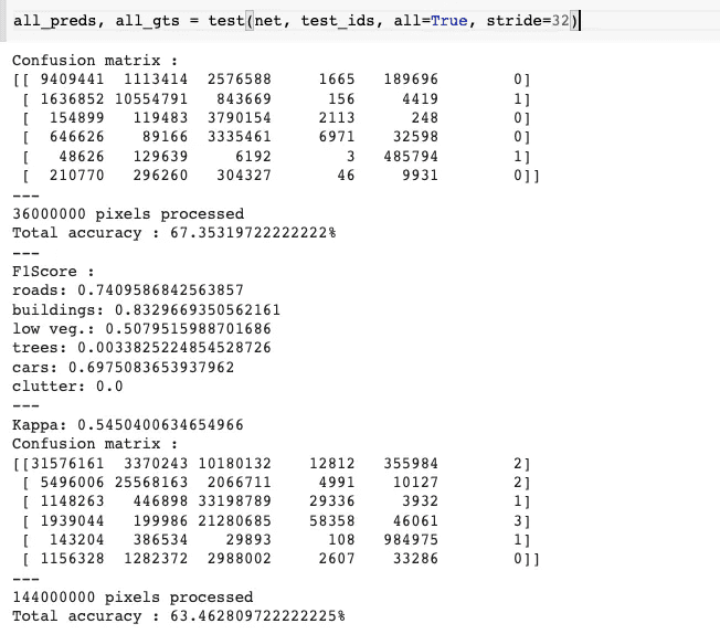
Finally, with an accuracy of 63%, we tested and trained our CNN utilizing VGG16 weights and a segnet architecture.
If you wish to view the Colab notebook, click the link below.
https://colab.research.google.com/drive/1lk2hG3LO8ndgaLGrCXPkcNwZ4cu8fS7E?authuser=2#scrollTo=mObJEW8mBF8Z&uniqifier=2
Google Colaboratory
I hope this article was informative and provided you with the details you required. If you have any questions while reading the blog, message me on Instagram or LinkedIn.For any kind of work related to Machine Learning Development you can contact me at helpmeanubhav@gmail.com
Thank You…
Random Erasing is a new data augmentation method for training the convolutional neural network (CNN).
Random Erasing
Contents:
Introduction to Random Erasing
Steps to achieve Random Erasing
Intraining, Random Erasing randomly selects a rectangle region in an image and erases its pixels with random values. In this process, training images with various levels of occlusion are generated, which reduces the risk of over-fitting and makes the model robust to occlusion. Random Erasing is parameter learning free, easy to implement, and can be integrated with most of the CNN-based recognition models.
Albeit simple, Random Erasing is complementary to commonly used data augmentation techniques such as random cropping and flipping, and yields consistent improvement over strong baselines in image classification, object detection, and person re-identification.
So, will perform step by step process and achieve Random Erasing from a well-known Potsdam dataset.
Dataset link:
Let’s hop in,
Step 1: To use Google Colab, the company’s most popular data science tool, we must first join in using our Google accounts. To make advantage of the GPU capabilities, we are utilizing Google Colab.
Step 2: Once we have the Colab in our possession, we mount the drive so that we may use the data that is on it. The corresponding photo is shown below.
Colab
Step 3: We will now download the dataset directly to the disc. The corresponding photo is shown below. The snippet below shows how to get data from a source and unzip it into a certain directory.
Dataset
Step 4: After receiving the dataset, I’ll download the relevant packages, import them into the colab, and then proceed with the processing. The corresponding photo is shown below.
Packages
Step 5: For our Potsdam dataset, we will use the random erasing function from Pytorch itself. So, in essence, we’ll create another Random Erasing dataset and utilize it for additional training. As a result, we are creating and saving the dataset in a particular place.
Step 6: Here, we will visualize the just-created random erasing dataset. The relevant photo is shown below. Let’s first examine if we can get the dataset and figure out what’s going on. Scikit-Image is what we’re using to manipulate images. We must create a color palette that can transfer the label id to its RGB color since the ISPRS dataset is stored with ground truth in the RGB format. To convert from numbers to colors and vice versa, we construct two helper functions.
The above code snippet gives output like the below image.
Step 7: Here, At this point, we need to define a bunch of utils function for the smooth processing
Step 8: Now we are loading the dataset, We define a PyTorch dataset (torch.utils.data.Dataset) that loads all the tiles in memory and performs random sampling. Tiles are stored in memory on the fly. The dataset also performs random data augmentation (horizontal and vertical flips) and normalizes the data in [0, 1].
So, we have defined a class and within it, data augmentation functions like flip, rotate, etc. Below is the snippet for the same.
Step 9: Now, the time comes for network definition for CNN, We can now define the Fully Convolutional network based on the SegNet architecture. We could use any other network as a drop-in replacement, provided that the output has dimensions (N_CLASSES, W, H) where W and H are the sliding window dimensions (i.e. the network should preserve the spatial dimensions).
Step 10: We can now instantiate the network using the specified parameters. By default, the weights will be initialized using the policy.
Step 11: We download and load the pre-trained weights from VGG-16 on ImageNet. This step is optional but it makes the network converge faster. We skip the weights from VGG-16 that have no counterpart in SegNet.
Below is the output of the above snippet.
Step 12: Now, we load the network on GPU. Follow the below link till Step 5, Link for GPU in the Colab:
https://www.geeksforgeeks.org/how-to-run-cuda-c-c-on-jupyter-notebook-in-google-colaboratory/
How To Run CUDA C/C++ on Jupyter notebook in Google Colaboratory - GeeksforGeeks
What is CUDA? CUDA is a model created by Nvidia for a parallel computing platform and application programming interface…
www.geeksforgeeks.org
And then write below code snippet.
Step 13: Now below is the code snippet with output for Cuda for training the CNN.
Step 14: Check the image below to see if the GPU is active.
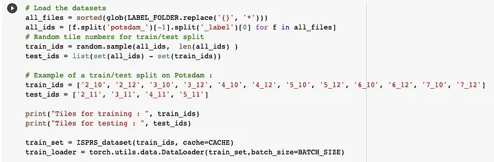
Step 15: Now we establish a train/test divide. You must modify the code to gather all filenames if you wish to utilize another dataset. In our scenario, the demo has a fixed train/test split.
Step 16: We are now designing the optimizer. We use the standard Stochastic Gradient Descent algorithm to optimize the network’s weights. The encoder is trained at half the learning rate of the decoder, as we rely on the pre-trained VGG-16 weights.
Step 17: Let’s progressively raise once the network has trained for two epochs. The loss plot and an example inference are updated on the matplotlib graph on a regular basis.
Step 18: Now that the training has ended, we can load the final weights and test the network using a reasonable stride, e.g. half or a quarter of the window size. Inference time depends on the chosen stride, e.g. a step size of 32 (75% overlap) will take ~30 minutes, but no overlap will take only one minute or two.
Finally, with an accuracy of 63%, we tested and trained our CNN utilizing VGG16 weights and a segnet architecture.
If you wish to view the Colab notebook, click the link below.
https://colab.research.google.com/drive/1lk2hG3LO8ndgaLGrCXPkcNwZ4cu8fS7E?authuser=2#scrollTo=mObJEW8mBF8Z&uniqifier=2
Google Colaboratory
I hope this article was informative and provided you with the details you required. If you have any questions while reading the blog, message me on Instagram or LinkedIn.For any kind of work related to Machine Learning Development you can contact me at helpmeanubhav@gmail.com
Thank You…
Random Erasing is a new data augmentation method for training the convolutional neural network (CNN).
Random Erasing
Contents:
Introduction to Random Erasing
Steps to achieve Random Erasing
Intraining, Random Erasing randomly selects a rectangle region in an image and erases its pixels with random values. In this process, training images with various levels of occlusion are generated, which reduces the risk of over-fitting and makes the model robust to occlusion. Random Erasing is parameter learning free, easy to implement, and can be integrated with most of the CNN-based recognition models.
Albeit simple, Random Erasing is complementary to commonly used data augmentation techniques such as random cropping and flipping, and yields consistent improvement over strong baselines in image classification, object detection, and person re-identification.
So, will perform step by step process and achieve Random Erasing from a well-known Potsdam dataset.
Dataset link:
Let’s hop in,
Step 1: To use Google Colab, the company’s most popular data science tool, we must first join in using our Google accounts. To make advantage of the GPU capabilities, we are utilizing Google Colab.
Step 2: Once we have the Colab in our possession, we mount the drive so that we may use the data that is on it. The corresponding photo is shown below.
Colab
Step 3: We will now download the dataset directly to the disc. The corresponding photo is shown below. The snippet below shows how to get data from a source and unzip it into a certain directory.
Dataset
Step 4: After receiving the dataset, I’ll download the relevant packages, import them into the colab, and then proceed with the processing. The corresponding photo is shown below.
Packages
Step 5: For our Potsdam dataset, we will use the random erasing function from Pytorch itself. So, in essence, we’ll create another Random Erasing dataset and utilize it for additional training. As a result, we are creating and saving the dataset in a particular place.
Step 6: Here, we will visualize the just-created random erasing dataset. The relevant photo is shown below. Let’s first examine if we can get the dataset and figure out what’s going on. Scikit-Image is what we’re using to manipulate images. We must create a color palette that can transfer the label id to its RGB color since the ISPRS dataset is stored with ground truth in the RGB format. To convert from numbers to colors and vice versa, we construct two helper functions.
The above code snippet gives output like the below image.
Step 7: Here, At this point, we need to define a bunch of utils function for the smooth processing
Step 8: Now we are loading the dataset, We define a PyTorch dataset (torch.utils.data.Dataset) that loads all the tiles in memory and performs random sampling. Tiles are stored in memory on the fly. The dataset also performs random data augmentation (horizontal and vertical flips) and normalizes the data in [0, 1].
So, we have defined a class and within it, data augmentation functions like flip, rotate, etc. Below is the snippet for the same.
Step 9: Now, the time comes for network definition for CNN, We can now define the Fully Convolutional network based on the SegNet architecture. We could use any other network as a drop-in replacement, provided that the output has dimensions (N_CLASSES, W, H) where W and H are the sliding window dimensions (i.e. the network should preserve the spatial dimensions).
Step 10: We can now instantiate the network using the specified parameters. By default, the weights will be initialized using the policy.
Step 11: We download and load the pre-trained weights from VGG-16 on ImageNet. This step is optional but it makes the network converge faster. We skip the weights from VGG-16 that have no counterpart in SegNet.
Below is the output of the above snippet.
Step 12: Now, we load the network on GPU. Follow the below link till Step 5, Link for GPU in the Colab:
https://www.geeksforgeeks.org/how-to-run-cuda-c-c-on-jupyter-notebook-in-google-colaboratory/
How To Run CUDA C/C++ on Jupyter notebook in Google Colaboratory - GeeksforGeeks
What is CUDA? CUDA is a model created by Nvidia for a parallel computing platform and application programming interface…
www.geeksforgeeks.org
And then write below code snippet.
Step 13: Now below is the code snippet with output for Cuda for training the CNN.
Step 14: Check the image below to see if the GPU is active.
Step 15: Now we establish a train/test divide. You must modify the code to gather all filenames if you wish to utilize another dataset. In our scenario, the demo has a fixed train/test split.
Step 16: We are now designing the optimizer. We use the standard Stochastic Gradient Descent algorithm to optimize the network’s weights. The encoder is trained at half the learning rate of the decoder, as we rely on the pre-trained VGG-16 weights.
Step 17: Let’s progressively raise once the network has trained for two epochs. The loss plot and an example inference are updated on the matplotlib graph on a regular basis.
Step 18: Now that the training has ended, we can load the final weights and test the network using a reasonable stride, e.g. half or a quarter of the window size. Inference time depends on the chosen stride, e.g. a step size of 32 (75% overlap) will take ~30 minutes, but no overlap will take only one minute or two.
Finally, with an accuracy of 63%, we tested and trained our CNN utilizing VGG16 weights and a segnet architecture.
If you wish to view the Colab notebook, click the link below.
https://colab.research.google.com/drive/1lk2hG3LO8ndgaLGrCXPkcNwZ4cu8fS7E?authuser=2#scrollTo=mObJEW8mBF8Z&uniqifier=2
Google Colaboratory
I hope this article was informative and provided you with the details you required. If you have any questions while reading the blog, message me on Instagram or LinkedIn.For any kind of work related to Machine Learning Development you can contact me at helpmeanubhav@gmail.com
Thank You…